In this post we'll give a very brief introduction to what principal component analysis can accomplish, and then look at one of scikit-learn's PCA tools applied to some face image data.
We'll import what we need here.
%matplotlib inline
import numpy as np
from scipy import misc # for image reading and manipulation
from sklearn.decomposition import RandomizedPCA # the PCA module we'll use
import matplotlib.pyplot as plt
import fnmatch # for finding files
import os # for finding files
A brief line example
We'll start off by applying PCA to model the set of points below by a line, and talk a bit about what PCA is doing in this case.
In the next block of code, we'll generate some points by randomly offsetting points from the line y= 1.5 x + 0.5. The particular line won't be important for us; we're just interested in what's going on visually.
x = np.linspace(0,1,100)
y = 1.5*x + 0.5 + np.random.normal(0,0.1,size=100)
plt.figure(figsize=(2,4))
plt.scatter(x,y)
plt.xlim(0,1)
plt.ylim(0,2);

The points were constructed for this example so that they would all be clearly near a line, with a small offsets in other directions.
Principal component analysis (PCA) is used to find the "best" linear coordinate system to describe a set of points. As usual, the notion of best requires clarification. Vaguely, PCA tries to minimize the error coming from the lengths of orthogonal projections from the points to the subspaces of the candidate coordinate spaces. This is a bit different from the optimization done in usual linear regression, which we can talk about in another post.
An advantage of PCA is that we can obtain a ranking of the axes in the new coordinate system. The axes can be ordered by how much of the variance they explain in the data (i.e. whether the points are spread out a lot or a little along that axis). This is useful, because we can decide to throw out some of the axes. If the data does not vary much along an axis, then disregarding that axis does not lose much information about the data. This insight allows us to effectively project our data to a lower dimension space without losing much information.
For example, in our linear-looking set of points above, PCA can be used to find the two "best" directions for describing the data. We expect one of the directions to match the linear-looking aspect of our data, and explain most of the spread of the points. We expect the other direction to match the offset-looking aspect of our data.
We will train a PCA-based model with 2 components (i.e. dimensions) and see what it gets us.
model = RandomizedPCA(n_components = 2)
model.fit(np.c_[x,y])
Below, we plot the points again, this time with the new axes drawn in red. The first axis found by PCA is drawn as a solid red line. As noted above, this axis follows the main linear spread of the points. The second axis is drawn as a dotted red line, and distance along this axis explains the orthogonal offset from the first axis.
# resize for a useful aspect ratio
plt.figure(figsize=(2,4))
plt.xlim(0,1)
plt.ylim(0,2)
# v1 and v2 are the vectors found by PCA which best explain the directions in which the points vary
v1 = model.components_[0]
v2 = model.components_[1]
# we need to build lines from the vectors so we can plot the axes
# we add and subtract each vector from the data's mean to get a pair of points in line with each vector
pca_axis_1 = np.c_[model.mean_ + v1, model.mean_ - v1]
pca_axis_2 = np.c_[model.mean_ + v2, model.mean_ - v2]
# then we draw the line between the corresponding pairs of points
plt.plot(pca_axis_1[0], pca_axis_1[1], c="red", linewidth=3)
plt.plot(pca_axis_2[0], pca_axis_2[1], c="red", linestyle="--", linewidth=3)
# draw the original points
plt.scatter(x,y);

We can see that the model found a new coordinate system that seems to match the data well.
As discussed above in general, the interesting thing is that we can perform dimension reduction using these axes. Since the data doesn't spread much along the second axis (the dotted line), we could chose to disregard it. That is, we could project all of our points onto the first axis (the solid line), and still maintain most of the useful information about our original points.
In the next section, we'll reproduce a common example of applying PCA to face image data.
Face data set
We can think of the PCA example above as having found a "main direction" in which out points varied. Below, we're going to apply PCA to images of faces.
Instead of points in a plane, we will begin with several thousand pictures of faces. After preparing the images, they will be 33x33 gray-scale pixels for a total of 1089 pixels each. This means that each image is essentially a point in a space with 1089 many dimensions (one for how black-or-white each pixel is).
However, images of faces do not fill up the entirety of this 1089-dimension space. Nearly all of that "possible 33x33 images" space consists of what we can consider meaningless noise. For example, below is a random image in such a space.
plt.figure(figsize=(2,2))
plt.imshow(np.random.randint(0,255,size=(33,33)), cmap=plt.cm.gray)
plt.xticks(())
plt.yticks(());

Images that we consider meaningful contain a large amount of structure. There is a lot of correlation or symmetry in recognizabe images. This holds even more so for faces. Intuitively, we're talking about things like how bilateral symmetry means that the left and right sides of an image of a face will tend to contain similar colors, and consistency of skin color means that the forehead and cheeks will generally be similar as well.
This presence of structure means that the interesting images will occupy a much smaller region of the 1089-dimension image space. This is like our line example above, where most of the 2d plane did not contain any of our points, which occupied a small, (conveniently) linearly shaped region.
We will use PCA to find a smaller dimension linear space which still captures a lot of information about faces.
To begin, we need to load our images so that we can work with them. We will be using part of the Labeled Faces in the Wild data set.
# this is the relative path to the directory where I extracted the data
base_dir = "../faces2/"
# the data is grouped into folders according to the subject in the photo
# recursively look through the folders for .jpg files
face_jpgs = []
for root, dirnames, filenames in os.walk(base_dir):
    for filename in fnmatch.filter(filenames, '*.jpg'):
        face_jpgs.append(os.path.join(root, filename))
# print how many photos we found
print len(face_jpgs)
Here's the first image we find from the data set. The images come in color, but we will only use a gray-scale version of each.
plt.imshow(misc.imread(face_jpgs[0], flatten=True), cmap=plt.cm.gray);

We can see that the data set is already preprocessed a bit. Each image has been altered a bit to center and align the face.
Reading in and preparing the images
We will do another step or two of processing to make the data a bit more manageable. We will focus just on the face, cropping down to the middle of the image. We will also resize the image down.
The original images are 250x250 color roughly shoulder-up images, and we will end up with 33x33 gray-scale images of just the faces.
For example, next we show what will happen to the image above. We will also record some information about the sizes for convenience later.
# get the image file and read it as a gray-scale image
img = misc.imread(face_jpgs[0], flatten=True)
# record the original width and height
orig_w, orig_h = img.shape
scale = 0.4
# crop and downsize the image
sample_face = misc.imresize(img[orig_w/3:2*orig_w/3,orig_h/3:2*orig_h/3], scale)
# record the new width and height
im_shape = sample_face.shape
# plot the example face
plt.figure(figsize=(2,2))
plt.imshow(sample_face, cmap=plt.cm.gray)
plt.xticks(())
plt.yticks(());

Now let's read them in. We will only use 1/3 of the files, because we're pretending that we're working on a cheap laptop and don't want to wait long.
num_faces = len(face_jpgs)/3
# compute the total number of pixels as width * height
num_pixels = np.product(sample_face.shape)
# prepare a blank numpy array to fill with the image data
faces = np.zeros((num_faces, num_pixels))
for i in xrange(num_faces):
    img = misc.imread(face_jpgs[i], flatten=True)
    faces[i] = misc.imresize(img[orig_w/3:2*orig_w/3,orig_h/3:2*orig_h/3], scale).reshape(num_pixels)
Now our faces matrix has rows corresponding to the images. We've flattened each image into a 1-d vector (row) to fit into the PCA model more easily. This just means we'll need to reshape things later when we want to display images.
Training the model
Next we'll train our PCA model. We'll use 15^2 = 225 components. That is, we'll only apply PCA to get a 225-dimension space of "directions". Implicitly, this means we are already deciding to disregard 1089 - 225 = 864 many dimensions. We'll see later that we could probably throw out even more. The way PCA works will automatically choose the "least informative" axes to throw out for us.
model = RandomizedPCA(n_components = 15**2)
model.fit(faces)
Our model now contains 225 many vectors in the original 1089-dimension image space. These 225 many vectors were selected as the best directions for explaining the spread of our face images within the original space. So, we can think of these 225 many vectors as the main "face directions".
Since these vectors can still be viewed as points in the original image space, we can plot them to get an idea of the "face directions" they represent. We do this next.
The images which do the most for explaining the spread of our data will appear near the top of what we're about to show. The images farther down can be thought of as explaining less frequent variations from a "typical" face. Vaguely, the images lower down have more to do with the subtleties and details of particular faces rather than the overall "face-ness".
plt.figure(figsize=(10,10))
for i in xrange(len(model.components_)):
    plt.subplot(15,15,i+1)
    plt.imshow(model.components_[i].reshape(im_shape), cmap=plt.cm.gray)
    plt.xticks(())
    plt.yticks(())
plt.subplots_adjust(wspace=0.1, hspace=0.1)
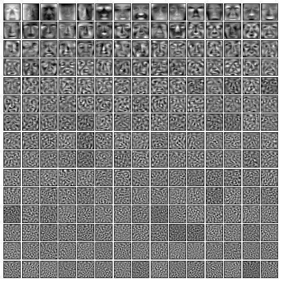
Any face image in our set can be roughly described as some linear combination of these images (offset from the average face). In this sense, the above faces are basis vectors for a new coordinate system centered at the average of our face image data.
Of course, this cannot completely reproduce a face, because we have thrown out a lot of dimensions which contained some (but not much) information. However, because the disregarded dimensions represent directions along which our data is not spread out much, ignoring them means that our reproductions will only be off by very small amounts.
What does it let us do?
Being able to describe the faces in terms of linear combinations of these 225 images means that we can project face images down into a 225-dimension space and still retain most of the information we care about.
We can think of this as determining a mapping from the 1089-dimension "image space" to the 225-dimension "face space". The nice thing about this mapping is that it preserves a lot of information. This should be contrasted, for example, with just dropping all but 225 many pixels from each image.
Let's look at an example of reconstructing a face using these "face directions".
The photo we will work with is the following image of G. W. Bush.
gwb_number = 4350
plt.figure(figsize=(2,2))
plt.imshow(faces[gwb_number].reshape(im_shape), cmap=plt.cm.gray)
plt.xticks(())
plt.yticks(());

We'll begin by taking this photo and mapping it into the "face space" to get a vector of weights for each of the 225 "face directions" above. Then we'll have a loop go over the first 15 axes/vectors/faces selected by PCA, and add the information for each one, displaying the image at each step. The result should be a series of photos that gradually shift from a generic face toward a recognizable photo of G. W. Bush.
# the index of a photo of G. W. Bush
face_number = 4350
# map the image to a weight vector
face_component_weights = model.transform(faces[face_number])[0]
# plot the result of adding one "direction" at a time, for the first 15 directions
plt.figure(figsize=(15,2))
partial_component_weights = np.zeros(model.n_components)
for i in xrange(15):
    # add another component's weight
    partial_component_weights[i] += face_component_weights[i]
    plt.subplot(1,15,i + 1)
    # map the "face-space" vector back to "image-space"
    partial_face = model.inverse_transform(partial_component_weights)
    # plot it
    plt.imshow(partial_face.reshape(im_shape),cmap=plt.cm.gray)
    plt.xticks(())
    plt.yticks(())

That was just the first 15 of the 225 directions found by PCA. Below, we'll continue similarly.
This time we show the images after each addition of 15 components. That is, we show the generic face, then the face reconstructed with the first 15 components, then with the first 30, then 45, etc.
face_component_weights = model.transform(faces[gwb_number])[0]
plt.figure(figsize=(15,2))
partial_component_weights = np.zeros(model.n_components)
for i in xrange(model.n_components):
    partial_component_weights[i] += face_component_weights[i]
    if i%15==0:
        plt.subplot(1,15,i/15 + 1)
        partial_face = model.inverse_transform(partial_component_weights)
        plt.imshow(partial_face.reshape(im_shape),cmap=plt.cm.gray)
        plt.xticks(())
        plt.yticks(())

We see that with all 225 dimensions accounted for, we've very recognizably reproduced the original image. It even appears that we could have stopped a bit earlier, using fewer dimensions. This isn't terribly surprising since we chose the number 225 arbitrarily.
Scikit-learn's PCA models have methods for telling us the amount of variance explained by each axis, and generally one would choose the number of components (i.e. dimensions or directions) based on how much variance is alright to ignore. We've chosen not to do that here and instead just look at the visual results.
From here, it would be reasonable to use our reduced dimensionality data to train other models more easily. This is a common use of PCA: projecting data down to smaller spaces so that it is easier to visualize or work with in other models. For example, we could use our new space to train a classifier or cluster similar faces. This would be easier to do with our 225-dimension or even smaller space than with the original 1089-dimension space.
But, we'll stop here and have coffee.
plt.figure(figsize=(7,2))
face_1 = faces[2393]
face_2 = faces[942]
plt.subplot(1,7,1)
plt.imshow(face_1.reshape(im_shape),cmap=plt.cm.gray)
plt.xticks(())
plt.yticks(())
for i in xrange(5):
    plt.subplot(1,7,i+2)
    face_mix = face_1 + i*(face_2 - face_1)/4.0
    plt.imshow(face_mix.reshape(im_shape),cmap=plt.cm.gray)
    plt.xticks(())
    plt.yticks(())
plt.subplot(1,7,7)
plt.imshow(face_2.reshape(im_shape),cmap=plt.cm.gray)
plt.xticks(())
plt.yticks(());
