In this post, we'll talk about how the "face directions" we found in our other post about principal component analysis (PCA) and faces can be useful for automatically locating faces within an image.
We'll handle the imports and file loading here and then start talking. We're loading and preparing the images like in the other post.
%matplotlib inline
import numpy as np
from scipy import misc # for image reading and manipulation
from sklearn.decomposition import RandomizedPCA # the PCA module we'll use
import matplotlib.pyplot as plt
import fnmatch # for finding files
import os # for finding files
# this is the relative path to the directory where I extracted the data
base_dir = "../faces2/"
# the data is grouped into folders according to the subject in the photo
# recursively look through the folders for .jpg files
face_jpgs = []
for root, dirnames, filenames in os.walk(base_dir):
    for filename in fnmatch.filter(filenames, '*.jpg'):
        face_jpgs.append(os.path.join(root, filename))
# print how many photos we found
print len(face_jpgs)
# crops down to the middle square of the image, where the face typically is
# and resizes to 33 x 33 pixels
def reshape_and_crop(img):
    orig_w, orig_h = img.shape
    scale = (33,33)
    return misc.imresize(img[orig_w/3:2*orig_w/3,orig_h/3:2*orig_h/3], scale)
# get the image file and read it as a gray-scale image
img = misc.imread(face_jpgs[0], flatten=True)
# crop and downsize the image
sample_face = reshape_and_crop(img)
# record the new width and height
im_shape = sample_face.shape
print im_shape
# plot the example face
plt.figure(figsize=(2,2))
plt.imshow(sample_face, cmap=plt.cm.gray)
plt.xticks(())
plt.yticks(());
num_faces = len(face_jpgs)
# compute the total number of pixels as width * height
num_pixels = np.product(sample_face.shape)
# prepare a blank numpy array to fill with the image data
faces = np.zeros((num_faces, num_pixels))
for i in xrange(num_faces):
    img = misc.imread(face_jpgs[i], flatten=True)
    faces[i] = reshape_and_crop(img).reshape(num_pixels)
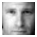
Quick summary of the data
An example of the cropped, resized images which we will work with can be seen above.
We've just built a matrix faces whose rows correspond to images from our face data set. The images (2d arrays of pixel info) were flattened into 1d vectors in order to accomplish this. This is just done to feed things into our PCA model more easily, and just requires that we reshape things appropriately when we want to show images again.
Training the model
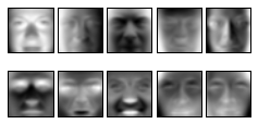
Now we'll train the model. This time we'll use just 10 components.
As a quick recap of what we discussed in the other post, this roughly means that we will ask PCA to find the 10 most significant face-like images that we can use to represent images of faces. These form a good collection of images that we can mix together to try to draw an arbitrary face.
n_components = 10
model = RandomizedPCA(n_components = n_components)
model.fit(faces)
Here's the 10 principal components or "face directions" we found.
plt.figure(figsize=(4,2))
for i in xrange(len(model.components_)):
    plt.subplot(2,5,i+1)
    plt.imshow(model.components_[i].reshape(im_shape), cmap=plt.cm.gray)
    plt.xticks(())
    plt.yticks(())
plt.subplots_adjust(wspace=0.1, hspace=0.1)
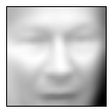
A random face
For fun, we'll randomly construct a face. We choose 10 random weightings, one for each of the above components, and then we use the model to recover an image. This should help suggest a bit why the 10 principal components above help to build out a whole space of faces.
The image we are about to make is a random face, built by randomly combining the principal components of faces we found. This is not a face that exists in our data set. It is also not just one of the above components.
We'll randomly pick weights uniformly between -1000 and 1000, though it would make more sense to choose a range determined from the actual data (for example by considering the variance in each of the "face directions" above).
# select a random set of weights for the "face directions" above
random_vector = np.random.uniform(-1000,1000,10)
# use the model to recover an image
random_face = model.inverse_transform(random_vector)
# plot the "random face"
plt.figure(figsize=(2,2))
plt.imshow(random_face.reshape(im_shape), cmap=plt.cm.gray)
plt.xticks(())
plt.yticks(());
Some notions of difference
Next, we'd like to move toward the point of this post. We are going to try to find a face after it's been superimposed onto another image.
Roughly, our strategy will be to slide a window around an image to obtain many smaller images, and measure how far those smaller images are from "face space".
To quantify how far a given image is from "face space", we'll use a simple distance function. Viewing images as vectors in some euclidean space $\mathbb{R}^\text{number of pixels}$, this is just the usual euclidean distance
def dist(p,q):
    return np.linalg.norm(p-q)
We expect this distance to be close to 0 for images which contain typical faces. This is because images containing faces should be very close to their projections into "face space", so most pixels should not change much under projection.
The next two examples help understand this point a bit better.
First, we'll take a picture of Bill Clinton's face, use the model to project it to "face space", and plot the image formed by taking the difference of these pictures.
After that, we'll do the same with a random image.
# plotting function to save space later
def plot_helper(p):
    v = model.transform(p)
    v_inv = model.inverse_transform(v)
    plt.figure(figsize=(6,2))
    # plot original face
    plt.subplot(1,3,1)
    plt.imshow(p.reshape(im_shape), cmap=plt.cm.gray)
    plt.xticks(())
    plt.yticks(())
    # plot the projection
    plt.subplot(1,3,2)
    plt.imshow(v_inv.reshape(im_shape), cmap=plt.cm.gray);
    plt.xticks(())
    plt.yticks(())
    # plot the difference
    plt.subplot(1,3,3)
    plt.imshow((abs(p-v_inv)).reshape(im_shape), cmap=plt.cm.gray);
    plt.xticks(())
    plt.yticks(());
    print "Distance from image to projection:", dist(p, v_inv)
bill_number = 1234
bills_face = faces[bill_number]
plot_helper(bills_face)
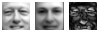
Notice that the projection has a lot of similarity with Bill's face. In the difference picture (the rightmost one), the darker spots correspond to pixels where the is not much difference between Bill's face and the projection. The distance of about 700 captures this relatively small difference across the image.
Contrast this with the random image example below.
p = np.random.uniform(0,255,num_pixels)
plot_helper(p)
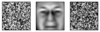
In this case, the projection (the middle image) is not very similar to the original image (left). The difference image (right) consequently has more lighter spots overall, corresponding to many pixels where there is substantial difference between the original and the projection. The large distance captures this dissimilarity.
Faces in a random image
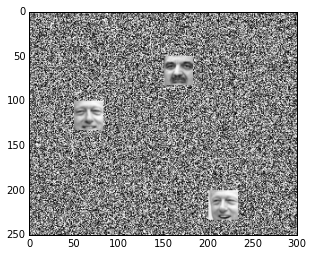
We'll now superimpose some faces onto an image of random noise, and show how we can find it with the strategy we outlined above.
Here's a random 250 x 300 image with some faces superimposed.
random_image = np.random.uniform(0,255,(250,300))
random_image[100:100+33,50:50+33] = faces[bill_number].reshape(33,33)
random_image[50:50+33,150:150+33] = faces[42].reshape(33,33)
random_image[200:200+33,200:200+33] = faces[1233].reshape(33,33)
plt.imshow(random_image, cmap=plt.cm.gray);
A window class
To help carry out our strategy of sweeping a window across the image to look for Bill, we'll make a Python class so we can get a window object that behaves how we'd like.
We'll just put the code here and then get back to the application.
The main interesting function in this class will be the step function, which advances our window around the image, and automatically handles repositioning the window when it reaches the edge of the image.
We will also have a draw function that plots the boundary of the window for us.
class Window:
    def __init__(self, width, height, parent_width, parent_height, step_size = 1):
        self.width = width
        self.height = height
        self.parent_width = parent_width
        self.parent_height = parent_height
        self.step_size = step_size
        self.x = 0
        self.y = 0
    def topright(self):
        return [self.x+self.width, self.y]
    def topleft(self):
        return [self.x,self.y]
    def bottomright(self):
        return [self.x+self.width, self.y+self.height]
    def bottomleft(self):
        return [self.x, self.y+self.height]
    def step(self):
        if self.x + self.width + self.step_size <= self.parent_width:
            self.x += self.step_size
            return True
        elif self.y + self.height + self.step_size <= self.parent_height:
            self.x = 0
            self.y += self.step_size
            return True
        else:
            return False
    def image(self, arr):
        return arr[self.x:self.x+self.width,self.y:self.y+self.height]
    def draw(self):
        top = np.c_[self.topleft(),self.topright()]
        right = np.c_[self.topright(),self.bottomright()]
        bottom = np.c_[self.bottomright(),self.bottomleft()]
        left = np.c_[self.bottomleft(),self.topleft()]
        plt.plot(top[1],top[0],linewidth=2)
        plt.plot(right[1],right[0],linewidth=2)
        plt.plot(bottom[1],bottom[0],linewidth=2)
        plt.plot(left[1],left[0],linewidth=2)
Automatically finding faces
Now we'll carry out the strategy, searching for Bill's face in the random image by sweeping our window across it and computing projection distances.
We've chosen in the code below to draw a window if we see that the project distance is less than 1000. We hand-chose this number to be large enough that would work, but not so large as to capture other random images. Remember that above, we saw that the image of Bill's face had a distance of around 700 from it's projection, while the random noise had a larger distance from its projection.
# show the background image, so we can draw windows on it
# image plotting reverses the axes, so we need to fuss around with xlim,ylim a bit
plt.imshow(random_image, cmap=plt.cm.gray);
plt.xlim(0,random_image.shape[1])
plt.ylim(random_image.shape[0],0)
# set the window info
width = height = 33
step_size = 10
window = Window(width, height, random_image.shape[0], random_image.shape[1], step_size)
# slide the window around the image
while True:
    # get the subpicture the window sees
    p = misc.imresize(window.image(random_image),im_shape).reshape(num_pixels)
    # project it into "face space"
    v = model.transform(p)
    v_inv = model.inverse_transform(v)
    # compute the info about how the projection differs
    d = dist(p, v_inv)
    # if the window doesn't change much under projection, draw the window's boundary
    if d < 1000:
        window.draw()
    # advance to next window or quit if we're done
    if not window.step():
        break
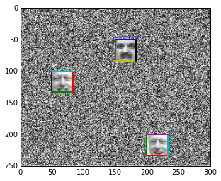
We see that we've located the positions of the faces. The windows have drawn multi-colored boundary boxes.
We've cheated in a few ways here to make things work, so we should talk about how, and about the shortcomings of this method.
Problems with generalizing
The 3 face images we used in the example above came from the training set, and the background is fairly special. We also hand selected the window size knowing how big the face images should be.
These issues present obstacles to generalizing the method, because we won't generally have such special images and backgrounds.
The fact that we used faces from the training set is not such a big deal, since once we have trained on enough faces, most face images should be close enough to the "face space" to be below a reasonable threshold.
The more interesting problem is with alternative backgrounds, and possibly identifying a window as containing a face when it does not.
Notice that the following all-black image has an even lower distance (about 450) to its "face space" projection than Bill's face did earlier (about 700).
p = np.zeros(num_pixels)
plot_helper(p)
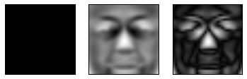
Despite clearly not being a face, the original image (left) is closer to its projection (middle) than Bill's face was.
This is possible in part because our training face images were close-cropped, gray-scale, and fairly low resolution. This means that areas like the forehead and cheeks look like large, bland, consistent patches.
Consequently, the principal components can be used to reconstruct bland images (like the black square), except for some differences near the eyes, nose, and mouth. Since the eyes, nose, and mouth occupy relatively few pixels, the overall distance is not very large. This can be seen in the difference image (right) above, where the majority of the image is very dark, except for some small bright regoins. This corresponds to an overall small difference, with relatively few pixels having a large difference.
To account for this, we could try using wider-cropped color photos, including more than just the immediate face. This would force non-face images to have more differences in the area surrounding what should be the head. Increased resolution could also help to detect more subtle facial features around the face, introducing more opportunities for differences to be detected.
We could also try using more components or some other notion of similarity, instead of the euclidean distance we are using. For example, weighting the differences near the typical eye, nose, and mouth positions would help to rule out the case above. Essentially, this would be a departure from the PCA, and a movement toward more domain-influenced feature-selection.
For now, we can just also require that the variance of an image is above some threshold, so that we avoid bland (likely non-face) images.
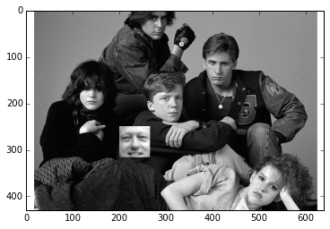
Mess with the bull
We'll close by trying to find a face in this piece of artwork. This will demonstrate the generalization problems above a bit more.
bfclub = misc.imread("../faces2/bfclub.png", flatten=True)
# insert Bill
width = height = 66
bfclub[250:250+66,200:200+66] = misc.imresize(faces[bill_number].reshape(im_shape),(66,66))
plt.imshow(bfclub, cmap=plt.cm.gray);
We'll run our window strategy to search for faces. In principle, we could expect to find any of them, but we'll see that's more difficult than it might seem.
Notice that we're also already cheating, only looking at window sizes agreeing with Bill's face image. In general, we would have to also search over a variety of window widths and heights, if we didn't already know what size image to look for.
# show the background image, so we can draw windows on it
plt.imshow(bfclub, cmap=plt.cm.gray);
plt.xlim(0,bfclub.shape[1])
plt.ylim(bfclub.shape[0],0)
# set the window info
# width and height are set above during Bill-imposition.
step_size = 10
window = Window(width, height, bfclub.shape[0], bfclub.shape[1], step_size)
# slide the window around the image
while True:
    # get the subpicture the window sees
    p = misc.imresize(window.image(bfclub),im_shape).reshape(num_pixels)
    # project it into "face space"
    v = model.transform(p)
    v_inv = model.inverse_transform(v)
    # compute the info about how the projection differs
    d = dist(p, v_inv)
    var = np.var(p)
    # if the window doesn't change much under projection, draw the window's boundary
    if d < 800 and var > 2000: # <--- we also check the variance this time
        window.draw()
    # advance to next window or quit if we're done
    if not window.step():
        break
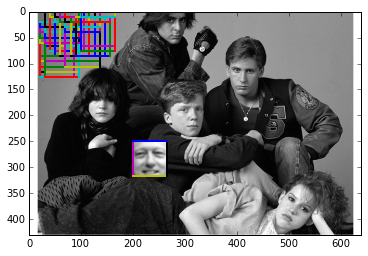
We've found Bill, but things are strange.
Despite also trying to search including the variance as a criterion, we've still selected a large number of "blank" squares in the top left. Trying to decrease the distance threshold or increase the variance threshold doesn't work, so we would need to keep trying other methods.
We've also failed to locate any other face. This happens for a few reasons, having mainly to do with the subtle size and pose problems. That is, the other faces are not oriented and sized well-enough to match our training data, so they are not close enough to our "face space".