In this post, we'll follow up on some of the suggestions for improvement we mentioned in part 1 of our discussion on finding faces using principal component analysis (PCA). This post assumes some familiarity with the previous post.
In this part, we use color images, more components, and let our windows (for searching subimages) vary in size as well. We get a bit better performance (i.e. locate some faces) in the final example at the bottom of this post.
As usual, we'll import everything and load the images to get started. There are a few minor changes to account for the color images.
Newer stuff and discussion will start in the next section.
%matplotlib inline
import numpy as np
from scipy import misc # for image reading and manipulation
from sklearn.decomposition import RandomizedPCA # the PCA module we'll use
import matplotlib.pyplot as plt
import fnmatch # for finding files
import os # for finding files
# this is the relative path to the directory where I extracted the data
base_dir = "../faces2/"
# the data is grouped into folders according to the subject in the photo
# recursively look through the folders for .jpg files
face_jpgs = []
for root, dirnames, filenames in os.walk(base_dir):
    for filename in fnmatch.filter(filenames, '*.jpg'):
        face_jpgs.append(os.path.join(root, filename))
# print how many photos we found
print len(face_jpgs)
# crops down to the middle square of the image, where the face typically is
# and resizes to 33 x 33 pixels by default
def reshape_and_crop(img, scale=(33,33)):
    orig_w, orig_h, orig_d = img.shape
    return misc.imresize(img[orig_w/3:2*orig_w/3, orig_h/3:2*orig_h/3, :], scale)
# a helper function, since we will shot images frequently
def show(img, dimensions=(33,33,3)):
    # we need to cast to uint8 for color images to show correctly
    plt.imshow(img.astype(np.uint8).reshape(dimensions))
    # remove tick marks
    plt.xticks(())
    plt.yticks(())
This time, we will read the images with the default setting flatten=False, so that we maintain the color.
For the purpose of making the images look a bit better when displayed, we'll also run everything through this simple filter we're about to define. It shifts and stretches the color range in the image to more fully use the range of colors available.
def stretch_colors(img):
    lo = np.min(img)
    hi = np.max(img - lo)
    return (img - lo)*(255.0/max(hi,0.001))
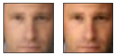
# get the image file and read it as a gray-scale image
img = misc.imread(face_jpgs[0])
# crop and downsize the image
sample_face = reshape_and_crop(img)
# record the new width and height
im_shape = sample_face.shape
print im_shape
plt.figure(figsize=(4,2))
# plot the example face
plt.subplot(1,2,1)
show(sample_face)
# plot the filtered example face
plt.subplot(1,2,2)
show(stretch_colors(sample_face))
This time, because we want to use more components, we're going to use fewer images from the data set to avoid memory problems. These trade-offs will continue until you get me that new computer you totally want to get for me.
We're inaccurately still calling the number of coordinates in an image num_pixels, though now there are three entries per pixel, because of the 3 color channels (i.e. red, green, blue values at each pixel, rather than a single luminosity value).
num_faces = len(face_jpgs)/10
# compute the total number of pixels as width * height * (3 color channels)
num_pixels = np.product(sample_face.shape)
# prepare a blank numpy array to fill with the image data
faces = np.zeros((num_faces, num_pixels))
for i in xrange(num_faces):
    img = misc.imread(face_jpgs[i])
    face = reshape_and_crop(img)
    p = face.reshape(num_pixels)
    faces[i] = p[:]
Everything is loaded, so we'll get to the newer stuff and discussion.
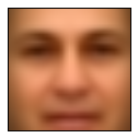
The mean face
This time, we're going to incorporate distance to the mean face as a criteria for deciding whether a window contains a face. This is an easy thing to compute and helps a bit.
Here we'll just compute the mean face (the average of all of the images in our training set) and show it.
mean_face = np.zeros(num_pixels)
for i in xrange(num_faces):
    mean_face += faces[i]/num_faces
plt.figure(figsize=(2,2))
show(stretch_colors(mean_face))
Training the model
We'll train the model with 225 components this time. The increased number of components will make it easier for actual face images to be closer to the "face space". Of course, some non-face images will now be closer as well (since, after all, we are increasing the size of the "face space"). But we hope that the actual faces gain more by this change than the non-faces.
n_components = 225
model = RandomizedPCA(n_components = n_components)
model.fit(faces)
Though we've chosen 225 components, we'll just show the first 15 below to give a sense of what we've found.
plt.figure(figsize=(10,2))
for i in xrange(15):
    plt.subplot(1,15,i+1)
    show(stretch_colors(model.components_[i]))
plt.subplots_adjust(wspace=0.001, hspace=0.001)

Notice that because we are using color images, this time the components incorporate some color information.
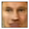
A random face
Like in the other post, we'll randomly construct a face to help give an impression of what the "face space" consists of.
As a quick explanation, the image we are about to make is a random face built by combining the principal components above. This is not a face that exists in our data set. It is also not just one of the above components.
This time we will randomly pick weights uniformly, using ranges determined by the variance explained in each component's direction.
# get a reasonable range of weights for each component
stds = (model.explained_variance_)**(0.5)
# select a random set of weights for the "face directions" above
random_vector = np.random.uniform(-stds,stds,n_components)
# use the model to recover an image
random_face = model.inverse_transform(random_vector)
# plot the "random face"
plt.figure(figsize=(2,2))
show(stretch_colors(random_face))
Notions of similarity
Like in the previous post, we will make use of the distance from images to their projection into "face space". This time, we will also make use of the distance to the mean_face we defined above, and the overall variance within the image.
Here's the distance function we'll use, followed by another helper function for some plotting.
After these blocks of code, we'll show an example.
def dist(p,q):
    return np.linalg.norm(p-q)
# plotting function to save space later
def plot_helper(p):
    v = model.transform(p)
    v_inv = model.inverse_transform(v)
    plt.figure(figsize=(6,2))
    # plot original face
    plt.subplot(1,3,1)
    #show(p)
    show(stretch_colors(p))
    # plot the projection
    plt.subplot(1,3,2)
    #show(v_inv)
    show(stretch_colors(v_inv))
    # plot the difference
    plt.subplot(1,3,3)
    show(abs(p-v_inv))
    print "Distance from image to projection:", dist(p, v_inv)
    print "Distance from image to mean face:", dist(p, mean_face)
    print "Variance in image:", np.var(p)
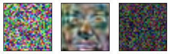
Here's the example. We'll keep using Bill Clinton's face. In this post, we will keep track of
- the distance from the image to its projection in "face space" (i.e. the distance between the original image and the best image that can be reconstructed using the 225 principal components we found above)
- the distance from the image to the mean face we found above
- the variance within the image
bill_number = 1234
bills_face = faces[bill_number]
plot_helper(bills_face)
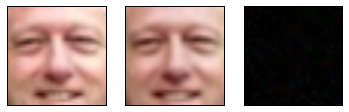
The left image is the original picture, the middle is the projection, and the rightmost one is a display of the difference between the images.
To quickly describe why we expect these measurements to be useful:
- Face-like images should generally be close to their projections into "face space", so this distance should be smaller than for most images.
- Face-like images should generally be close to the mean face image. Including this helps to separate out non-face images which happen to be close to linear combinations of components in strange ways (e.g. close to "face space" because of abnormally high weights on some components).
- Variance is included to help account for examples like the solid black square being close to "face space". Face images should have a variance away from 0, but also not so large as random images.
The 2nd and 3rd points could be expanded in yet more detailed work in the following way. We could compute the mean and variance in each principal component ("face direction") we found earlier, rather than just for overall images. This would let us build a description of how atypical the image is not just overall, but in terms of the weight of each component considered individually.
However, the three measurements above will suffice for now.
For comparison with the Bill Clinton face above, here's a random image, its projection and difference images, and its measurements.
p = np.random.uniform(0,255,num_pixels)
plot_helper(p)
And for more comparison, here is a black square.
p = np.zeros(num_pixels)
plot_helper(p)

Notice, unfortunately, that the black square is still closer to "face space" than the real Bill Clinton face, for similar reasons to the ones we discussed in the previous post. However, notice that the distance to the mean is much larger, and the variance is much smaller than for Bill's face.
A window class
Like in the previous post, here is our Window class. It lets us get a Window object which makes it easier to loop through the sub-images of a given image. Again, our purpose in the end of this post is to locate faces within a given image.
The interesting functions are:
- step, which advances the window through the parent image.
- image, which returns the sub-image determined by the window and the given image.
- draw, which plots the window edges on the parent image.
class Window:
    def __init__(self, width, height, parent_width, parent_height, step_size = 1):
        self.width = width
        self.height = height
        self.parent_width = parent_width
        self.parent_height = parent_height
        self.step_size = step_size
        self.x = 0
        self.y = 0
    def topright(self):
        return [self.x+self.width, self.y]
    def topleft(self):
        return [self.x,self.y]
    def bottomright(self):
        return [self.x+self.width, self.y+self.height]
    def bottomleft(self):
        return [self.x, self.y+self.height]
    def step(self):
        if self.x + self.width + self.step_size <= self.parent_width:
            self.x += self.step_size
            return True
        elif self.y + self.height + self.step_size <= self.parent_height:
            self.x = 0
            self.y += self.step_size
            return True
        else:
            return False
    def image(self, arr):
        return arr[self.x:self.x+self.width,self.y:self.y+self.height]
    def draw(self):
        top = np.c_[self.topleft(),self.topright()]
        right = np.c_[self.topright(),self.bottomright()]
        bottom = np.c_[self.bottomright(),self.bottomleft()]
        left = np.c_[self.bottomleft(),self.topleft()]
        plt.plot(top[1],top[0],linewidth=2)
        plt.plot(right[1],right[0],linewidth=2)
        plt.plot(bottom[1],bottom[0],linewidth=2)
        plt.plot(left[1],left[0],linewidth=2)
Automatically finding faces
To quickly recap our strategy from the last post, we will sweep a window over an image to get lots of sub-images, and measure how "facelike" each sub-image is.
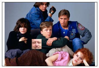
We'll carry out this strategy on the chef-d'oeuvre below.
bfclub = misc.imread("../faces2/bfclub.png")
bfclub = np.delete(bfclub,obj=3,axis=2) #remove alpha channel
# insert Bill
width = height = 66
p = misc.imresize(faces[bill_number].reshape(im_shape),(width,height,3))
bfclub[250:250+66,200:200+66] = p
show(bfclub, dimensions=bfclub.shape)
We will search over a few window sizes (from 40x40 pixels to 70x70), and draw a window when the sub-image it determines has
- distance to projection < 700
- distance to mean < 3500
- variance > 3000
These numbers were selected by hand, based on some examples similar to ones we saw above.
# show the background image, so we can draw windows on it
show(bfclub, dimensions=bfclub.shape)
plt.xlim(0,bfclub.shape[1])
plt.ylim(bfclub.shape[0],0)
# set the window info
width = height = 40
step_size = 10
# loop over window sizes
for k in xrange(7):
    #print "Step", k, "width x height:", width, height
    window = Window(width, height, bfclub.shape[0], bfclub.shape[1], step_size)
    # slide the window around the image
    while True:
        # get the subpicture the window sees
        p = misc.imresize(window.image(bfclub),im_shape).reshape(num_pixels)
        # project it into "face space"
        v = model.transform(p)
        v_inv = model.inverse_transform(v)
        # compute the info about how the projection differs
        d_proj = dist(p, v_inv)
        d_mean = dist(p, mean_face)
        var = np.var(p)
        # if the window's image satisfies the constraints, draw it
        if d_proj < 700 and d_mean < 3500 and var > 3000: # <--- we also check the variance this time
            window.draw()
        # advance to next window or quit if we're done
        if not window.step():
            break
    # increase window size for next pass
    width += 5
    height += 5
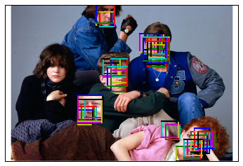
We've performed better this time, thanks to the additional measurements we've taken, extra components and colors, and range of window sizes we've allowed. We've still missed a face, possibly because of the bangs. Surprisingly, we seem to have found Molly Ringwald's face in the bottom right. This (along with many of the partial-face including boxes near the faces) is actually an indication of a weakness in our strategy. These windows pass our test likely because they contain large skin-toned patches.
In the future, we could try the suggestions made above. Namely, accounting more in-depth for how each image's weights sit across the principal components individually.