Interpreting neural networks in terms of hyperplanes
Matt Luther 🏠 🐦 🔗
In this post, we'll implement a neural network and demonstrate that it can correctly separate some simple non-linearly-separable data sets. While demonstrating this, we'll talk about how we can interpret the weight matrices and nonlinear functions involved in computing the layers of the network.
In particular, we'll visualize the first layer of weights and hidden activations. We'll interpret the weight matrix as determining a family of hyperplanes through the input space, and interpret the hidden activations in terms of distances of the inputs to those hyperplanes. Since we'll focus on 2d inputs for easier visualization, the hyperplanes will just be lines.
%matplotlib inline
import numpy as np
import matplotlib.pyplot as plt
A quick overview of neural networks
Neural networks are a computational model inspired by simple models of neuron behavior in the brain. Discussions often embrace this view, describing neural networks as directed, weighted graphs whose nodes carry out some computation, analogous to neurons being activated based on the strength of their connections to other neurons. The computations involved in these models can be described using matrix multiplication, vector addition, and nonlinear transformations. We will skip right to this formulation.
The network is provided with an input vector X (or matrix X whose rows are each input vectors). The network then repeatedly carries out the following basic computation.
$$ f\left(\text{(Input vector)} \cdot \text{(Weight matrix)} + \text{(bias vector)}\right) $$where $f$ is a nonlinear function, typically applied elementwise. In our implementation, we will use a "leaky rectifier"
$$ f(x) = \cases{\array{x &\text{ when } x\geq0\\x/100 &\text{ when } x<0}} $$This is a slight modification of the function $\max(0,x)$, which can be interpreted as measuring how much larger x is than 0. In one of the sections below, we will instead use the absolute value function $g(x)=|x|$, which can be thought of as giving the distance of x from 0.
The output of the first application of this computation is the "first hidden layer". Applying this computation again, with the first hidden layer as the input, yields the values of the "second hidden layer" and so on. The "hidden" name comes from these layers being neither of the exposed input or output layers.
The weight matrix and bias vectors are allowed to vary (and almost certainly do) in each application of this basic computation to obtain the next layer. The nonlinear function, however, is typically selected in advance and does not change.
This basic computation is repeated some number of times to compute all "hidden layers", and then a final computation without applying $f$ is done to produce the output of the network.
Since multiplication by a matrix followed by addition of a vector is just an affine transformation, we can describe the full computation involved in obtaining a neural network's output as an alternating composition of affine and nonlinear functions:
$$ X_\text{in} \overset{\text{Affine}_1}{\longmapsto} \circ \overset{\text{Nonlinear}}{\longmapsto} \text{Hidden}_1 \overset{\text{Affine}_2}{\longmapsto} \cdots \overset{\text{Nonlinear}}{\longmapsto} \text{Hidden}_k \overset{\text{Affine}_k}{\longmapsto} y_\text{out} $$To train the network, we fix the number and dimensions of the matrices and bias vectors, but otherwise consider the affine functions (i.e. the entries of the corresponding weight matrix and bias vector) to be parameters, and we try to optimize against some loss function which compares $y_\text{out}$ to a known correct $y_\text{target}$ corresponding to $X_\text{in}$. A standard way to carry out this optimization is to randomly initialize the parameters, then use gradient descent and train on batches of known input-output pairs.
Intuition
The intuition we'll suggest throughout this post is to think of affine transformations as computing many signed, scaled distances to hyperplanes (e.g. planes in 3d space, lines in 2d space, or points in 1d space).
This is one of the possible interpretations of linear and affine transformations, and follows from the definition of matrix multiplication in terms of dot products, and the relation between dot products and scalar projections. That is, since
$$ \frac{v\cdot w}{||w||} $$is the signed length of the orthogonal projection of $v$ onto $w$, we can also think of $v\cdot w$ as a signed, scaled distance from $v$ to the hyperplane with normal vector $w$.
For example, the equation
$$ \left(\matrix{1&0}\right) \cdot \left(\matrix{\frac{\sqrt{2}}{2}&-1\\ \frac{\sqrt{2}}{2}&1}\right) = \left(\matrix{\frac{\sqrt{2}}{2}&-1}\right) $$can be interpreted as computing the following.
- The distance from $(1,0)$ to the line through the origin whose normal vector is $(\frac{\sqrt{2}}{2},\frac{\sqrt{2}}{2})$ is $\frac{\sqrt{2}}{2}$ units in the positive direction (i.e. in the normal vector's direction). The line in this case is y = -x.
- The distance from $(1,0)$ to the line through the origin whose normal vector is $(-1,1)$ is $1$ scaled units in the negative direction (i.e. opposite the normal vector's direction). The scaling of the units comes from the magnitude of the normal vector. That is, the actual (signed) distance from $(1,0)$ to this line is $\frac{-1}{\sqrt{(-1)^2 + (1)^2}} = \frac{\sqrt{2}}{2}$. The line in this case is y = x. We didn't have to worry about scaling in the first case, because $(\frac{\sqrt{2}}{2},\frac{\sqrt{2}}{2})$ has length 1.
The addition of a bias vector to the result of a computation like this is equivalent to shifting the lines before computing the distances. That is, bias vectors allow us to use lines that do not pass through the origin.
Throughout this post, we will generally discuss 2d spaces and distances to lines. In higher dimensions, this naturally generalizes to distances to hyperplanes.
With the exception of the final output layer, the network will follow each such computation by a nonlinear function. So, in our view, neural networks repeatedly combine and nonlinearly alter signed, scaled distances to hyperplanes in order to compute the hidden layers, and finish by computing signed, scaled distances to hyperplanes which divide the last hidden layer's space.
One of the things we'll see below is an example of how the choice of nonlinear function affects this interpretation, and also how this choice can impact the architecture of the network required to learn a task.
A neural network class
In this section, we import our neural network class. This is a large chunk of code, so the implementation can be found here
Our class has a constructor which lets us specify the input size, number and size of hidden layers, output size (i.e. number of classes in the classification task), and the standard deviations for randomly initializing our weights and biases around 0. Given our interpretation of the computations in the network, the initialization of weights and biases is equivalent to randomly selecting hyperplanes passing near the origin for each layer of values. This emphasis on the origin should be kept in mind since it suggests doing things like normalizing the data. However, we won't normalize data in this post.
The remaining methods in our class are loss, train, and predict. Each allows us to operate on multiple inputs at once by passing the inputs as a 2d numpy array X whose rows are the individual inputs.
- The loss method computes output scores for each class, and if the expected class labels are provided as well, loss computes the gradients needed to update the network.
- The train method repeatedly calls loss and updates the network using the gradients.
- The predict method returns the predicted class labels. The predicted class for an input is defined to be the class with the highest score computed by loss.
from neural_net import Net
Some functions to help plotting
This section just defines some functions we will call repeatedly in the discussion below to plot things. This can be skipped since we'll discuss the plots as we produce them.
The first, plot_predictions, takes one of our Net objects and an input matrix X. It assumes the inputs are 2d and that there are 2 classes in the task. It produces a color-shaded plot to indicate how the network classifies each point in a region of the plane, and then scatters the inputs from X over this region.
The colors and markers parameters are used to help visualize the classes of the points in X.
def plot_predictions(n,X,colors,markers):
    # step size and limits for the meshgrid
    h = 0.01
    x_min, x_max = -1, 2
    y_min, y_max = -1, 2
    xx, yy = np.meshgrid(np.arange(x_min, x_max, h), np.arange(y_min, y_max, h))
    # predict values for each of the mesh points
    Z = n.predict(np.c_[xx.ravel(), yy.ravel()])
    # color parts of the plane according to the model predictions
    Z = Z.reshape(xx.shape)
    plt.contourf(xx, yy, Z, alpha=0.5, levels=[0,0.5,1], colors=["red","blue"])
    for i in xrange(len(X)):
        plt.scatter(X[i,0],X[i,1], s=100, c=colors[i], marker=markers[i])
The second, plot_weight_cuts, similarly takes a Net object and input matrix X, and also assumes 2d inputs. For each vector in the first weight matrix (equivalently, each node in the first hidden layer), it plots a region of the plane and draws the line corresponding to that vector of the weight matrix. Furthermore, it shades the "positive" and "negative" sides of the plane, relative to this line.
We'll discuss this more when we use it in later examples.
def plot_weight_cuts(n,X,colors,markers,subplot_dims=None):
    hidden_layer_size = n.weights[0].shape[1]
    if subplot_dims == None:
        subplot_dims = [1,hidden_layer_size]
        plt.figure(figsize=(hidden_layer_size*2,2))
    else:
        plt.figure(figsize=(subplot_dims[0],subplot_dims[1]))
    h = 0.01
    x_min, x_max = -1, 2
    y_min, y_max = -1, 2
    xx, yy = np.meshgrid(np.arange(x_min, x_max, h), np.arange(y_min, y_max, h))
    for i in xrange(hidden_layer_size):
        plt.subplot(subplot_dims[0],subplot_dims[1],i+1)
        plt.xlim((-1,2)), plt.ylim((-1,2)), plt.xticks((0,1)), plt.yticks((0,1))
        for j in xrange(len(X)):
            plt.scatter(X[j,0],X[j,1], s=100, c=colors[j], marker=markers[j])
        # predict values for each of the mesh points
        Z = np.dot(np.c_[xx.ravel(), yy.ravel()], n.weights[0][:,i]) + n.biases[0][i]
        Z = Z.reshape(xx.shape)
        # color parts of the plane according to the model predictions
        plt.contourf(xx, yy, Z, alpha=0.5, levels=[-20,0,20], colors=["black","white"])
The last one, plot_first_hidden_values, assumes that the first hidden layer has 2 nodes, and in this case computes and plots the first hidden layer's values for each input.
def plot_first_hidden_values(n,X,colors,markers):
    n.predict(X)
    for i in xrange(len(X)):
        print X[i], "-->", n.activations[0][i]
    plt.figure(figsize=(2,2));
    plt.xticks((0,1))
    plt.yticks((0,1))
    for i in xrange(len(X)):
        plt.scatter(n.activations[0][i,0],n.activations[0][i,1], c=colors[i], marker=markers[i], s=100);
Our example data
Here we just define our example data. We will design and train neural networks to classify the data in later sections.
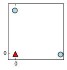
The matrix X consists of 4 row vectors, each of which is considered one input vector. The vector y contains the correct labels for the corresponding rows of X. This choice of X and y can be thought of as defining the xnor function, or truth table for logical equivalence.
We also define lists color and marker so that we can plot the input points with their classes more easily.
X = np.array([
        [0,0],
        [0,1],
        [1,0],
        [1,1]
    ])
y = np.array([
        1,
        0,
        0,
        1
    ])
colors = ["red" if v==0 else "lightblue" for v in y]
markers = ["^" if v==0 else "o" for v in y]
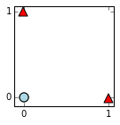
We'll plot these points and their classes now. The points with class 0 are drawn as red triangles, and the points with class 1 are drawn as blue circles.
plt.figure(figsize=(2,2))
plt.xticks((0,1))
plt.yticks((0,1))
for i in xrange(len(X)):
    plt.scatter(X[i,0],X[i,1], s=100, c=colors[i], marker=markers[i]);
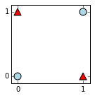
Notice that the 2 classes are not linearly separable. We'll see below that a neural network can learn to separate them.
Over the next few sections, we will compute some networks with hand-selected parameters, and then switch to using our Net object to automatically train and find parameters.
First, we'll use a simple, more easily interpretable case where our nonlinear function is the absolute value function, rather than the $f$ from above.
Constructing a network by hand with the absolute value function
In this section, we manually work out parameters for a network to separate the classes in the above example. The point is to develop some intuition about the role of a hidden layer computation.
Consider what we get if we map each input to its distance to the line y=x. This corresponds to taking a dot product with a single weight vector given by a unit normal vector $(-\frac{\sqrt{2}}{2},\frac{\sqrt{2}}{2})$ for this line, followed by elementwise application of the nonlinear absolute value function $g(x)=|x|$.
A picture might help to visualize the transformation.
plt.figure(figsize=(2,2))
plt.xticks((0,1))
plt.yticks((0,1))
for i in xrange(len(X)):
    plt.scatter(X[i,0],X[i,1], s=100, c=colors[i], marker=markers[i]);
xs = np.linspace(0,1,100)
plt.plot(xs,xs,c="black");
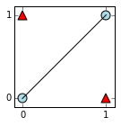
We can see that the blue circles would be sent to 0 (since they are on the line), and the red triangles would be sent to $\frac{\sqrt{2}}{2}$ (since that is their distance to the line).
The computation involved here is the following, where we view the inputs as a matrix whose rows are the individual inputs.
$$ g\left( \left(\matrix{0&0\\0&1\\1&0\\1&1}\right) \cdot \left(\matrix{-\frac{\sqrt{2}}{2}\\ \frac{\sqrt{2}}{2}}\right) + 0 \right) = g\left( \matrix{0\\ \frac{\sqrt{2}}{2}\\ -\frac{\sqrt{2}}{2}\\0} \right) = \left( \matrix{0\\ \frac{\sqrt{2}}{2}\\ \frac{\sqrt{2}}{2}\\0} \right) $$Geometrically, we can think of this transformation as folding the input space at the line, and just recording the distance from the fold.
This transformation maps each of the 2d inputs to a 1d space where they are linearly separable, for example by the point halfway between them at $\frac{\sqrt{2}}{4}$.
In the context of a neural network, the resulting linear separability means we could activate output nodes to correctly classify the inputs. For example, a single output node and a threshold for classification would work. However, in our setting, we want an output node for each of the 2 classes in the task, and we will interpret the prediction of the network (for each input) to be the index of the output node with the largest value. Based on the values we computed above, we can get a correct classification by computing these 2 output nodes to be the distances to the points $0$ and $\frac{\sqrt{2}}{2}$.
We demonstrate this computation (just an affine transformation) now. As a reminder
- the column vector on the left below corresponds to the list of (single node) hidden layer values for each of the original inputs.
- the second vector is the weight matrix for this final computation.
- the matrix we add corresponds to the bias vector for this computation, replicated across several rows since we are computing for multiple inputs at once.
We interpret the index of the maximum entry (in each row) as the prediction of the network. So, we see that the overall classification is correct.
$$ \left( \matrix{0&0\\0&1\\1&0\\1&1} \right) \overset{\text{Network}}{\longmapsto} \left( \matrix{0 & 1 \\ 1 & 0 \\ 1 & 0 \\ 0 & 1} \right) \overset{\text{Predict}}{\longmapsto} \left( \matrix{1 \\ 0 \\ 0 \\ 1} \right) $$We've just explained how a neural network with a single hidden node could learn to correctly classify these points if we use the absolute value function $g(x)=|x|$ as the nonlinear function in our network. To do this, we selected weights and biases by hand, using the interpretation in terms of distances to hyperplanes to guide us.
Why does that network work well?
The network we hand-constructed in the last section works well because its design matches well with the symmetries inherent in the data.
The fact that the affine transformation computes a signed distance to a hyperplane meshes well with the translation invariance of the classes. That is, we found a line such that the classes do not change as you move parallel to the line, and these parallel paths of motion correspond to level sets of our affine function.
Our use of the absolute value function meshes well with the reflective symmetry of the classes. That is, reflecting points over the line keeps classes consistent, and the symmetry of $|x|$ around 0 captures this.
This is an admittedly contrived example, but should be kept in mind since it indicates some basic strengths of networks with this nonlinear function.
This is a reasonable time to point out that, while we do not have to use $|x|$ as our nonlinear function, we did have to use some nonlinear function to classify this data. Notice that if we did not apply $g$ above, the hidden layer values would be the signed distances and so would not have been separable (according to their corresponding classes) by a point. This could not be corrected by just altering the number or dimensions of weight matrices, since a composition of affine transformations is still affine. A nonlinearity was necessary here.
When we actually train our network later via gradient descent, we'll use the nonlinear function $f$ we defined earlier rather than the absolute value function we just used, because $f$ is one of the more standard nonlinear functions in use. This is more general, for example because $f(x) + f(-x)$ approximates the absolute value function, and so two weight vectors in opposite directions (i.e. corresponding to the same line but with opposite "positive sides") accomplishes approximately the same thing as one line with $g$. With additional hidden nodes (i.e. additional weight vectors as columns in the weight matrix), we are able to use information related to distances to multiple hyperplanes through the input space.
Near the end of this post, we will see a different data set without such a strong relation to hyperplanes, and we'll show how a network could work there with some more effort.
Hand-selected parameters and the nonlinear function $f$
In this section, we'll switch back to the "leaky rectifier" function $f$ we defined at the start of this post. We will still hand-select weights and biases for our network to gain an understanding of how the network can classify the data. We are continuing to use the xnor example data from above. We'll also continue visualizing the lines involved in the computations.
This next code block initializes one of our Net objects with 2d input, 2 output classes, and a single hidden layer with 2 nodes. We then immediately set the weights and biases using hand-selected values.
Afterward, we will visualize the weights and biases to help explain where they come from. Essentially, this will be a demonstration of the comment at the end of the last section, where we said that $f(x) + f(-x)$ could be used in place of the absolute value function for a similar effect. For our first layer, we use two copies of the same line, but with opposite normal vectors. This gives us two values in the hidden layer. The 2nd set of weights adds these together, but is otherwise similar to the previous section.
n = Net(2,[2],2, std=1, bstd=1)
n.weights[0] = np.array([
        [-1,1],
        [1,-1]
        ])
n.biases[0] = np.array([0,0])
n.weights[1] = np.array([
        [1,-1],
        [1,-1]
        ])
n.biases[1] = np.array([0,1])
Note that numpy handles replicating our bias vectors into bias matrices when needed for computations involving multiple inputs at once.
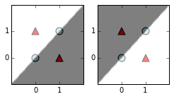
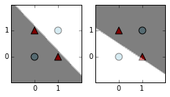
Below, we plot the lines corresponding to the first set of weight vectors (the columns of the weights[0] numpy array above). We use two separate plots, one for each weight vector. In these plots, we shade the plane white on the "positive side" of the line, and black on the "negative side" of the line. To explain a bit further: because the lines are defined by using the weight vector as the normal vector to the line, the line has a side coinciding with the direction of the weight vector. Points on the same side as the weight vector will have a positive dot product with the weight vector. Points on the opposite side will have negative dot products with the weight vector.
As described above, we are choosing two weight vectors in opposite directions, so that the corresponding lines are the same, but the positive and negative sides are reversed.
plot_weight_cuts(n,X,colors,markers)
Because we are using $f$ as our nonlinear function, the values of the first hidden layer will not be scaled positive distances to these lines (as it would be for $g$), but rather are signed, scaled distances to the lines, where negative distances are additionally scaled down by 100 (this follows from the definition of $f$).
We compute and plot these activations now.
plot_first_hidden_values(n,X,colors,markers)
This involves 2 dimensions this time, but we can still see a folding effect we've created. Both blue circles are mapped to (0,0), with the red triangles further away because of their distances to the 2 lines. We can see that in this transformed space, the classes are linearly separable.
In particular, if we add the 2 hidden values for each input, we get $(0,0.99,0.99,0)$ and have a situation analogous to the last section. This addition of components can be implemented as part of the matrix multiplication in computing the next layer (the outputs). This is how the 2nd set of weights for this section were constructed: we use weights analogous to the last section, apply them to both components and then add them together. This can be seen by working out the matrix multiplication.
Below, we show the output results computed by the network.
print n.activations[1]
Again, because the predictions are interpreted to be the indices of the maximum values, we get the correct labels:
print n.predict(X)
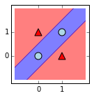
Finally, we'll close this section by showing a plot of the plane, shaded according to how points are classified by the network. Because we've taken advantage of how $f(x) + f(-x) \approx |x|$, we can again think of the transformations involved as folding the input plane along y=x, and then classifying points based on their distance from the fold. The network's use of this symmetry and the translation invariance we mentioned earlier is apparent in how the classification boundary forms a band centered along the line y=x.
plt.figure(figsize=(2,2))
plt.xticks((0,1))
plt.yticks((0,1))
plot_predictions(n,X,colors,markers)
In the next section, we'll start training networks instead of hand-selecting parameters.
Training networks
So far, we've demonstrated that there are possible selections of parameters that will work to correctly classify our example data. In the following sections, we let our network automatically discover parameters.
One hidden layer with 2 nodes
We'll start with a network having 1 hidden layer with 2 nodes. Even though we just showed a nice solution exists for this architecture, the network can have some trouble converging to an accurate solution because of the small number of parameters and poor initialization. So, we'll cheat and wrap the training in a loop that runs until the classification is correct.
is_good = False
while not is_good:
    n = Net(2,[2],2, std=1, bstd=1)
    n.train(X,y,X,y,num_iters=500,batch_size=0, learning_rate=0.1, learning_rate_decay=0.99);
    is_good = np.array_equal(n.predict(X),[1,0,0,1])
plot_predictions(n,X,colors,markers)
To relate things to our earlier discussion, below are plots of the lines and shadings determined by the first set of weight vectors, like in the previous section.
In many cases, the network will find a solution like ours from above. It can sometimes find alternate solutions based on the line y = 1-x instead. Also it is not critical that the lines coincide, so they are often roughly parallel but offset from each other.
plot_weight_cuts(n,X,colors,markers)
And here are the values of the first hidden layer, so we can see how the inputs have been transformed into linearly separable values.
plot_first_hidden_values(n,X,colors,markers)
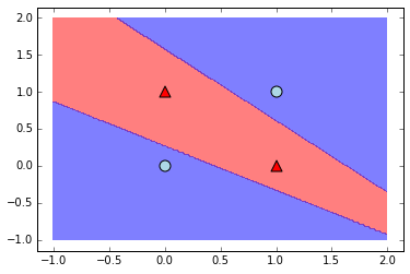
One hidden layer with 25 nodes
This next network will have 25 nodes in its hidden layer. We can interpret this as involving computations about 25 lines through the input space. This allows much more complex decision boundaries.
Since there are so many random lines initialized by the network, it's also more likely that some of them are useful. This makes it easier for the network to converge to an accurate solution. Since the complexity of this model is so high compared to this data set, we can get a variety of solutions.
n = Net(2,[25],2, std=1, bstd=1)
n.train(X,y,X,y,num_iters=500,batch_size=0, reg=0.001, learning_rate=0.1, learning_rate_decay=0.99);
print n.predict(X)
plot_predictions(n,X,colors,markers)
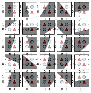
Next we'll plot the 25 lines and shaded planes corresponding to the first set of weight vectors.
For such a simple data set, this number of weight vectors is unnecessary, but it can be helpful to see how the variety enables the network to construct more complicated decision boundaries. Because the output layer computes many linear combinations of the activations associated to these lines, and because of our choice of $f$, we can (to some approximation) view an abundance of these linear cuts as providing our network with access to something like indicator functions for strips or rectangles in the plane.
plot_weight_cuts(n,X,colors,markers,subplot_dims=[5,5])
Because the hidden layer in this case would be 25-dimensional (one dimension for each line above), we won't plot those values.
Another example data set
We'll finish this post by quickly covering a new data set. We will once again hand-pick weights and biases to suggest how a neural network can learn to separate the classes. Afterward, we will train a network with a more complicated decision boundary.
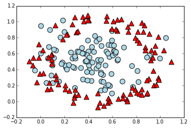
We'll construct and plot the data now.
n_samples = 200
X = np.zeros((n_samples,2))
y = np.zeros(n_samples)
# info for the normal distribution we use to build the central cluster of points
mu = 0.5
std = 0.2
# populates X and y
for i in xrange(n_samples/2):
    # cluster with label 0
    X[i] = np.random.normal(mu, std, (1,2))
    y[i] = 1
for i in xrange(n_samples/2,n_samples):
    # ring of points with label 1
    random_radius = np.random.uniform(0.4,0.6)
    random_angle = np.random.uniform()*2*np.pi
    x1_off = random_radius * np.cos(random_angle)
    x2_off = random_radius * np.sin(random_angle)
    X[i] = np.array([mu + x1_off, mu + x2_off])
    y[i] = 0
colors = ["red" if v==0 else "lightblue" for v in y]
markers = ["^" if v==0 else "o" for v in y]
for i in xrange(n_samples):
    plt.scatter(X[i,0],X[i,1],c=colors[i],marker=markers[i],s=100)
Hand-designing a network for this data
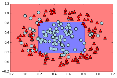
From the construction and visualization of the data, it's clear that a "correct" classification would be given by classifying everything inside a circle centered at $(0.5,0.5)$ as being class 1 (the blue circles), and everything outside this circle as being class 0 (the red triangles).
Based on the intuition developed in our earlier sections, we could expect to roughly approximate this by using distances to lines intersecting at the center of that circle (i.e. intersecting at $(0.5,0.5)$). Since we are still using networks with the nonlinear function $f$ we defined above, we could accomplish this with a network having 4 hidden nodes in a single hidden layer. Again, this is because the 4 hidden nodes correspond to 4 weight vectors, each determining a line. Since the $f(x)+f(-x)$ trick from earlier lets us roughly get the distance to a line from 2 weight vectors, we can use this network architecture to classify based on the distance to a pair of lines meeting at the center of the data. Our final output layer computation will be able to sum the distances to these lines. This means we can have the network classify based on something like the $\ell_1$ distance to the lines' intersection: this will be realized as a rectangular classification boundary.
We'll set the parameters of our network now by hand, and then show how well it predicts, plotting similar figures to above.
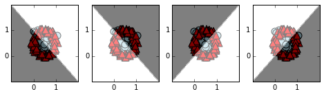
We won't discuss the choice of parameters in detail; they are a straightforward generalization from the earlier discussion where we wanted distance to a single line. This time we add the (scaled) distances for intersecting lines, as described in the paragraph above. The role of the 2nd set of weights and bias values is to let the classification be decided by whichever is the larger of
- the sum of the scaled distances to the lines
- 1.25 - the sum of the scaled distances to the lines (the particular value of 1.25 was just guessed)
n = Net(2,[4],2)
n.weights[0] = np.array([
        [1,-1,1,-1],
        [1,-1,-1,1]
        ])
n.biases[0] = np.array([-1,1,0,0])
n.weights[1] = np.array([
        [1,-1],
        [1,-1],
        [1,-1],
        [1,-1]
        ])
n.biases[1] = np.array([0,1.25])
Here's the accuracy of our network (the proportion of data set members it classifies correctly, 1 would be perfect classification).
print np.mean(n.predict(X) == y)
plot_predictions(n,X,colors,markers)
plt.xlim((-.2,1.2))
plt.ylim((-.2,1.2));
plot_weight_cuts(n,X,colors,markers)
Letting a network learn the parameters
We'll finish by training a network on this data set. If we mean-center the data, our network can sometimes find the solution we just gave in the last section. However, because of the small number of parameters and random initialization, it still has some difficulty. Instead, here we will just add more parameters and find an alternative solution.
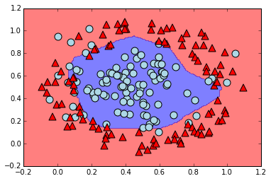
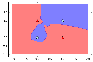
We will train a network with 2 hidden layers having 25 hidden nodes each. This will allow a more circular decision boundary, but because the data isn't cleanly separable, we shouldn't expect much better performance.
n = Net(2,[25,25],2,std=1,bstd=1)
n.train(X,y,X,y,num_iters=500,batch_size=0, reg=0.001, learning_rate=0.1, learning_rate_decay=0.99, verbose=False);
print "Accuracy:", np.mean(n.predict(X) == y)
plot_predictions(n,X,colors,markers)
plt.xlim((-.2,1.2))
plt.ylim((-.2,1.2));